PGE323M Reservoir Engineering III (Simulation)
import IPython.display
from IPython.core.display import HTML
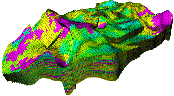
IPython.display.Image('images/sim.png', embed=True)

© UNISIM, Image Source
What is reservoir simulation?
- Understand flow and transport in our reservoirs to make engineering decisions
- Develop mathematical models to describe pressure, velocity, saturation, etc.
- Described by coupled, nonlinear partial differential equations (PDEs)
- Solution to PDEs can’t be found analytically – we are left with solving numerically
Reservoir simulators help us answer several questions
How should a field be developed to maximize economic recovery?
What is the best enhanced recovery scheme for the reservoir?
Why is the reservoir not behaving according to predictions made by previous engineering studies?
What is the ultimate economic recovery of the field?
What type of laboratory data is required?
Is it necessary to do physical model studies of the reservoir?
What is the best completion scheme for wells?
From what portion of the reservoir is the production coming?
Modeling and simulation
%%tikz --scale 1.0 --size 500,500 -f png
\tikzstyle{block} = [rectangle, draw, fill=blue!20,  node distance=3cm, text width=6em, text centered, rounded corners, minimum height=4em]
\tikzstyle{line} = [draw, -latex]
\node [block] (problem) {Engineering Problem};
\node [block, below of=problem] (model) {Mathematical Model};
\node [block, right of=model, node distance=5cm] (numerical) {Numerical Model};
\node [block, right of=problem, node distance=5cm] (solution) {Engineering Solution};
\path [line] (problem) -- (model);
\path [line] (model) -- (numerical);
\path [line] (numerical) -- (solution);

All steps in simulation are important
Conversion to mathematical model requires understanding physics
Fluid and rock properties of the reservoir
Laws that describe flow and transport (conservation of mass, energy, and momentum)
Numerical solution to the mathematical problem requires simplifications and approximations that are still accurate
Assume that fluid and rock properties are constant over a control volume
Transform non-linear PDEs into linear system of algebraic equations
Solve the system of equations
- Using the math solution to find an engineering solution requires economics, experience, and good decision-making skills
General idea
IPython.display.Image('images/res_to_block.png', embed=True)

- Break up the reservoir into individual "blocks", "grids", "cells", or "elements"
- Write algebraic equations for pressure, saturation, etc. each block
- Each block depends on the adjacent block equations so we get a system of linear equations
- Solve the system of equations. More blocks means more accuracy, but longer computation time
Simulation schematic
IPython.display.Image('images/sim_schematic.png', embed=True, width=500)

Conservation law...
{Rate In} - {Rate Out} = {Accumulation}
For each component (oil, gas, water, energy)
For each cell
Solving the PDEs that describe flow in porous media
- Equations come from a mass balance and implementing Darcy's law:
Complications
Coupled equations (water and oil)
PDEs (time and space – 1, 2 ,or 3D)
Variable properties (like permeability and porosity)
Approximations
$$ \begin{bmatrix} T_1 & -T_{1/2} & & \\ -T_{1/2} & T_2 & -T_{3/2} & \\ & -T_{3/2} & T_3 & -T_{5/2} \\ & & -T_{5/2} & T_4 \end{bmatrix} \left\lbrace \begin{matrix} P_1 \\ P_2 \\ P_3 \\ P_4 \end{matrix} \right\rbrace = \left\lbrace \begin{matrix} Q_1 \\ Q_2 \\ Q_3 \\ Q_4 \end{matrix} \right\rbrace $$What tools do I need to create my simulator?
- Write equations for fluid transport in porous media, rock/fluid properties, and conservation of mass, momentum, and energy
Use and perform error analysis of approximate numerical techniques to solve math problems
Root finding
Systems of equations
Interpolation, Integration, etc.
Solution to differential equations
- Develop computer programs to solve these massive numerical problems
Why can't I just use a commercial simulator (CMG, Eclipse) that someone smart already made?
- Great danger in using software if you don’t understand the fundamentals it was built on
- Simulators have lots of limitations. They can give very misleading results and only an understanding of the problem and mathematics will help your recognize when they do.
- Understanding the math and physics separates you from the technician
- Who knows you might be the smart person that creates the next commercial reservoir simulator
Categories of Reservoir Simulators
Commercial
CMG
Eclipse (Schlumberger)
Intersect (Schlumberger + Chevron)
Nexus (Halliburton)
In House
Empower (ExxonMobil)
Cheers (Chevron)
PSim (ConocoPhillips)
MoReS – (Shell)
Powers – (Saudi)
Academic
UT-CHEM (UT Chemical Flooding)
IPARS (UT Multiscale Simulation)
GPAS (UT compositional)
TOUGH2 (Lawrence Berkley National Labs)
