Faults and fractures at depth

import IPython.display
IPython.display.Image('images/strike_rake.png', width=400, embed=True)

© Cambridge University Press Zoback, Reservoir Geomechanics (Fig. 5.5, pp. 150)

Geographical coordinate system

%%tikz --size 400,400 -f png -l arrows.meta
\draw[line width=2pt, -latex] (0,0) -- (0,-5);
\draw[line width=2pt, -latex] (0,0) -- (5,0);
\draw[line width=2pt, -latex] (0,0) -- (3,3);
\draw[line width=2pt, dashed] (2,0) -- (3.5,1.5);
\draw[line width=2pt, dashed] (1.5,1.5) -- (3.5,1.5);
\draw[line width=2pt, dashed] (3.5,1.5) -- (3.5,2.5);
\draw[line width=2pt, dashed] (3.5,1.5) -- (0,0);
\draw[line width=2pt, color=red,-latex] (0,0) -- (3.5,2.5);
\draw[line width=2pt, dashed] (0,0) -- (-1.5,-1.5);
\draw[line width=2pt, dashed] (-1.5,-1.5) -- (2.,-1.5);
\draw[line width=2pt, dashed] (2.,-1.5) -- (3.5,0);
\draw[line width=2pt, dashed] (2.,-1.5) -- (0.,0.);
\draw[line width=2pt, dashed] (2.,-1.5) -- (2.,-2.5);
\draw[line width=2pt, color=red,-latex] (0.0,0.0) -- (2.,-2.5);
\draw[line width=2pt, color=red,-latex] (0.0,0.0) -- (0.75,-3.0);
\draw[->,line width=1pt] (2.3,1) arc (0:15:2);
\draw[->,line width=1pt,rotate around={60:(0,0)}] (2.7,-0.7) arc (5:-28:2);
\draw[->,line width=1pt] (1.7,-1.3) arc (5:-15:2);
\node[] (a) at (1.4,-1.35) {\Large $\gamma$};
\node[] (a) at (2.4,2) {\Large $\alpha$};
\node[] (a) at (1.95,1.1) {\Large $\beta$};
\node[] (a) at (3.3,3.3) {\Large $\mathbf{N}$};
\node[] (a) at (5.3,0.3) {\Large $\mathbf{E}$};
\node[] (a) at (1,-4.5) {\Large $\mathbf{D}(\mbox{own})$};
\node[color=red] (a) at (4.0,2.5) {\Large $S_1$};
\node[color=red] (a) at (2.5,-2.5) {\Large $S_2$};
\node[color=red] (a) at (1.2,-3.0) {\Large $S_3$};

$$ \mathbf{R}_G = \begin{bmatrix} \cos\alpha \cos\beta & \sin\alpha \cos\beta & -\sin\beta \\ \cos\alpha \sin\beta\sin\gamma - \sin\alpha\cos\gamma & \sin\alpha\sin\beta\sin\gamma + \cos\alpha\cos\gamma & \cos\beta\sin\gamma \\ \cos\alpha\sin\beta\cos\gamma + \sin\alpha\sin\gamma & \sin\alpha\sin\beta\cos\gamma - \cos\alpha\sin\gamma & \cos\beta\cos\gamma \end{bmatrix} $$

Interactive widget

import matplotlib.pyplot as plt
from mpl_toolkits.mplot3d import Axes3D
import numpy as np
from ipywidgets import interact, widgets

@interact(alpha_=widgets.IntSlider(min=0,max=360,step=10,value=20,description=r'$\alpha$'), 
          beta_=widgets.IntSlider(min=0,max=360,step=10,value=0,description=r'$\beta$'), 
          gamma_=widgets.IntSlider(min=0,max=360,step=10,value=0,description=r'$\gamma$'))
def create_plot(alpha_, beta_, gamma_):
    
    alpha = np.deg2rad(alpha_)
    beta = np.deg2rad(beta_)
    gamma = np.deg2rad(gamma_)

    soa1 = np.array([[0, 0, 0, 1, 0, 0], [0, 0, 0, 0, 1, 0],
                    [0, 0, 0, 0, 0, 1]])

    soa2 = np.array([[0, 0, 0, np.cos(alpha) * np.cos(beta), np.sin(alpha) * np.cos(beta), -np.sin(beta)], 
                     [0, 0, 0, np.cos(alpha) * np.sin(beta) * np.sin(gamma) - np.sin(alpha) * np.cos(gamma), np.sin(alpha) * np.sin(beta) * np.sin(gamma) + np.cos(alpha) * np.cos(gamma), np.cos(beta) * np.sin(gamma)], 
                    [0, 0, 0, np.cos(alpha) * np.sin(beta) * np.cos(gamma) + np.sin(alpha) * np.sin(gamma), np.sin(alpha) * np.sin(beta) * np.cos(gamma) - np.cos(alpha) * np.sin(gamma), np.cos(beta) * np.cos(gamma)]])

    X1, Y1, Z1, U1, V1, W1 = zip(*soa1)
    X2, Y2, Z2, U2, V2, W2 = zip(*soa2)
    fig = plt.figure(figsize=(8,8))
    ax = fig.add_subplot(111, projection='3d')
    ax.quiver(X1, Y1, Z1, U1, V1, W1, color='k', arrow_length_ratio=0.1, length=2, linewidths=3)
    ax.quiver(X2, Y2, Z2, U2, V2, W2, color='r', arrow_length_ratio=0.1, length=2, linewidths=3)
    ax.text(2, 0, 0, "$N$", color='k', fontsize=20)
    ax.text(0, 2, 0, "$E$", color='k', fontsize=20)
    ax.text(0, 0, 2, "$D$", color='k', fontsize=20)
    if (np.abs(U1[0] - U2[0]) >= 0.01):
        ax.text(2 * U2[0], 2 * V2[0], 2 * W2[0], "$S_1$", color='r', fontsize=20)
    if (np.abs(V1[1] - V2[1]) >= 0.01):
        ax.text(2 * U2[1], 2 * V2[1], 2* W2[1], "$S_2$", color='r', fontsize=20)
    if (np.abs(W1[2] - W2[2]) >= 0.01):
        ax.text(2 * U2[2], 2 * V2[2], 2 * W2[2], "$S_3$", color='r', fontsize=20)
    ax.view_init(200,-10)
    ax.set_axis_off()
    ax.set_xlim([-1.2, 1.2])
    ax.set_ylim([-1.2, 1.2])
    ax.set_zlim([-1.2, 1.2])
    plt.show()

Stress in geographical coordinate system

${}$

$$ \mathbf{S}_G = \mathbf{R}_G^T \mathbf{S} \mathbf{R}_G $$

Example: Strike-slip faulting

${}$

$$\mathbf{S}=\begin{bmatrix} 30 & 0 & 0 \\ 0 & 25 & 0 \\ 0 & 0 & 20 \end{bmatrix}$$

$$\quad\quad\quad$$

\begin{align} \alpha &= 0^{\circ} & \mbox{Azimuth of } S_{Hmax} \\ \beta &= 0^{\circ} & S_1 = S_{Hmax} \\ \gamma &= 90^{\circ} & S_2 = S_v \end{align}

$$ \mathbf{R}_G = \begin{bmatrix} 1 & 0 & 0 \\ 0 & 0 & 1 \\ 0 & -1 & 0 \end{bmatrix} $$

$$ \mathbf{S}_G = \begin{bmatrix} 30 & 0 & 0 \\ 0 & 20 & 0 \\ 0 & 0 & 25 \end{bmatrix} $$

Example: Normal faulting

${}$

$$\mathbf{S} = \begin{bmatrix} 30 & 0 & 0 \\ 0 & 25 & 0 \\ 0 & 0 & 20 \end{bmatrix}$$

$$\quad\quad\quad$$

\begin{align} \alpha &= 0^{\circ} & \mbox{Azimuth of } S_{hmin} \\ \beta &= -90^{\circ} & S_1 = S_v \\ \gamma &= 0^{\circ} & \end{align}

$$ \mathbf{R}_G = \begin{bmatrix} 0 & 0 & 1 \\ 0 & 1 & 0 \\ -1 & 0 & 0 \end{bmatrix} $$

$$ \mathbf{S}_G = \begin{bmatrix} 20 & 0 & 0 \\ 0 & 25 & 0 \\ 0 & 0 & 30 \end{bmatrix} $$

Example: Reverse faulting

${}$

$$\mathbf{S} = \begin{bmatrix} 30 & 0 & 0 \\ 0 & 25 & 0 \\ 0 & 0 & 20 \end{bmatrix}$$

$$\quad\quad\quad$$

\begin{align} \alpha &= 90^{\circ} & \mbox{Azimuth of } S_{Hmax} \\ \beta &= 0^{\circ} & S_1 = S_{Hmax} \\ \gamma &= 0^{\circ} & S_2 = S_{hmin} \end{align}

$$ \mathbf{R}_G = \begin{bmatrix} 0 & 1 & 0 \\ -1 & 0 & 0 \\ 0 & 0 & 1 \end{bmatrix} $$

$$ \mathbf{S}_G = \begin{bmatrix} 25 & 0 & 0 \\ 0 & 30 & 0 \\ 0 & 0 & 20 \end{bmatrix} $$

Example: Strike-slip faulting

${}$

$$\mathbf{S} = \begin{bmatrix} 60 & 0 & 0 \\ 0 & 40 & 0 \\ 0 & 0 & 35 \end{bmatrix}$$

$$\quad\quad\quad$$

\begin{align} \alpha &= 135^{\circ} & \mbox{Azimuth of } S_{Hmax} \\ \beta &= 0^{\circ} & S_1 = S_{Hmax} \\ \gamma &= 90^{\circ} & S_2 = S_{v} \end{align}

$$ \mathbf{R}_G = \begin{bmatrix} -\frac{1}{\sqrt{2}} & \frac{1}{\sqrt{2}} & 0 \\ 0 & 0 & 1 \\ \frac{1}{\sqrt{2}} & \frac{1}{\sqrt{2}} & 0 \end{bmatrix} $$

$$ \mathbf{S}_G = \begin{bmatrix} 47.5 & -12.5 & 0 \\ -12.5 & 47.5 & 0 \\ 0 & 0 & 40 \end{bmatrix} $$

Fault orientation

%%tikz --size 300,300 -f png
\node (myfirstpic) at (0,0) {\includegraphics[]{/Users/john/Documents/PGE334-ResGeomechanics/website/lectures/images/strike_rake.png}};
\draw[-latex, color=red, line width=4pt] (0.3,4.5) -- (3.3,1.7);
\draw[-latex, color=red, line width=4pt] (0.3,4.5) -- (3.3,6.4);
\draw[-latex, color=red, line width=4pt] (0.3,4.5) -- (1.3,8.4);
\node[color=red] (a) at (1.5,8.4) {\Large $\hat{\mathbf{n}}$};
\node[color=red] (a) at (3.0,6.8) {\Large $\hat{\mathbf{n}}_s$};
\node[color=red] (a) at (3.0,1.5) {\Large $\hat{\mathbf{n}}_d$};

© Cambridge University Press Zoback, Reservoir Geomechanics (Fig. 5.5, pp. 150)

${}$

$$\hat{\mathbf{n}} = \begin{bmatrix} -\sin(strike)\sin(dip) \\ \cos(strike)\sin(dip) \\ -\cos(dip) \end{bmatrix}$$

$$\quad\hat{\mathbf{n}}_s = \begin{bmatrix} \cos(strike) \\ \sin(strike) \\ 0 \end{bmatrix}\quad$$

$$\hat{\mathbf{n}}_d = \begin{bmatrix} -\sin(strike)\cos(dip) \\ \cos(strike)\cos(dip) \\ \sin(dip) \end{bmatrix}\quad$$

Fault traction and stress

${}$

Traction on fault plane

\begin{equation} \vec{t} = \mathbf{S}_G \cdot \hat{\mathbf{n}} \end{equation}

Normal stress to plane

\begin{equation} S_n = \vec{t}^\intercal \cdot \hat{\mathbf{n}} \end{equation}

Shear stress in dip direction

\begin{equation} \tau_d = \vec{t}^\intercal \cdot \hat{\mathbf{n}}_d \end{equation}

Shear stress in strike direction

\begin{equation} \tau_s = \vec{t}^\intercal \cdot \hat{\mathbf{n}}_s \end{equation}

Example: Strike-slip faulting

${}$

$$\mathbf{S}_G = \begin{bmatrix} 30 & -8.66 & 0 \\ -8.66 & 40 & 0 \\ 0 & 0 & 30 \end{bmatrix}$$

$$\quad\quad\quad$$

\begin{align} strike &= 60^{\circ} \\ dip &= 90^{\circ} \end{align}

$$\quad\hat{\mathbf{n}} = \begin{bmatrix} -0.866 \\ 0.5 \\ 0 \end{bmatrix}\quad$$

$$\quad\hat{\mathbf{n}}_s = \begin{bmatrix} 0.5 \\ 0.866 \\ 0 \end{bmatrix}\quad$$

$$\quad\hat{\mathbf{n}}_d = \begin{bmatrix} 0 \\ 0 \\ 1.0 \end{bmatrix}\quad$$

$$S_n = 40 \quad \tau_d = 0 \quad \tau_s = 8.66$$

Example: Normal faulting

${}$

$$\mathbf{S}_G = \begin{bmatrix} 4000 & 0 & 0 \\ 0 & 3000 & 0 \\ 0 & 0 & 5000 \end{bmatrix}$$

$$\quad\quad\quad$$

\begin{align} strike &= 45^{\circ} \\ dip &= 60^{\circ} \end{align}

$$\quad\hat{\mathbf{n}} = \begin{bmatrix} -0.612 \\ 0.612 \\ -0.5 \end{bmatrix}\quad$$

$$\quad\hat{\mathbf{n}}_s = \begin{bmatrix} 0.707 \\ 0.707 \\ 0 \end{bmatrix}\quad$$

$$\quad\hat{\mathbf{n}}_d = \begin{bmatrix} -0.3535 \\ 0.3535 \\ 0.866 \end{bmatrix}\quad$$

$$S_n = 3875 \quad \tau_d = -650 \quad \tau_s = -433$$

Example: Normal faulting

${}$

$$\mathbf{S}_G = \begin{bmatrix} 5000 & 0 & 0 \\ 0 & 4000 & 0 \\ 0 & 0 & 3000 \end{bmatrix}$$

$$\quad\quad\quad$$

\begin{align} strike &= 225^{\circ} \\ dip &= 60^{\circ} \end{align}

$$\quad\hat{\mathbf{n}} = \begin{bmatrix} 0.612 \\ -0.612 \\ -0.5 \end{bmatrix}\quad$$

$$\quad\hat{\mathbf{n}}_s = \begin{bmatrix} -0.707 \\ -0.707 \\ 0 \end{bmatrix}\quad$$

$$\quad\hat{\mathbf{n}}_d = \begin{bmatrix} 0.3535 \\ -0.3535 \\ 0.866 \end{bmatrix}\quad$$

$$S_n = 4125 \quad \tau_d = -650 \quad \tau_s = -433$$

Example: Revese faulting

${}$

$$\mathbf{S}_G = \begin{bmatrix} 2100 & -520 & 0 \\ -520 & 1500 & 0 \\ 0 & 0 & 1000 \end{bmatrix}$$

$$\quad\quad\quad$$

\begin{align} strike &= 120^{\circ} \\ dip &= 70^{\circ} \end{align}

$$\quad\hat{\mathbf{n}} = \begin{bmatrix} -0.814 \\ -0.470 \\ -0.342 \end{bmatrix}\quad$$

$$\quad\hat{\mathbf{n}}_s = \begin{bmatrix} -0.5 \\ 0.866 \\ 0 \end{bmatrix}\quad$$

$$\quad\hat{\mathbf{n}}_d = \begin{bmatrix} 0.2961 \\ -0.1710 \\ 0.9396 \end{bmatrix}\quad$$

$$S_n = 1441 \quad \tau_d = 161 \quad \tau_s = 488$$

Shear failure (slip on faults)

${}$

$$ \dfrac{\tau}{\sigma_n} = \mu $$

Coulomb failure function

$$ f = \tau - \mu \sigma_n \le 0 $$

Frictional strength of faults

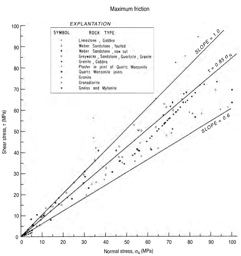
© Cambridge University Press Zoback, Reservoir Geomechanics (Fig. 4.23, pp. 126)

Induced seismicity

Fluid injection and seismicity at the Rocky Mountain Arsenal

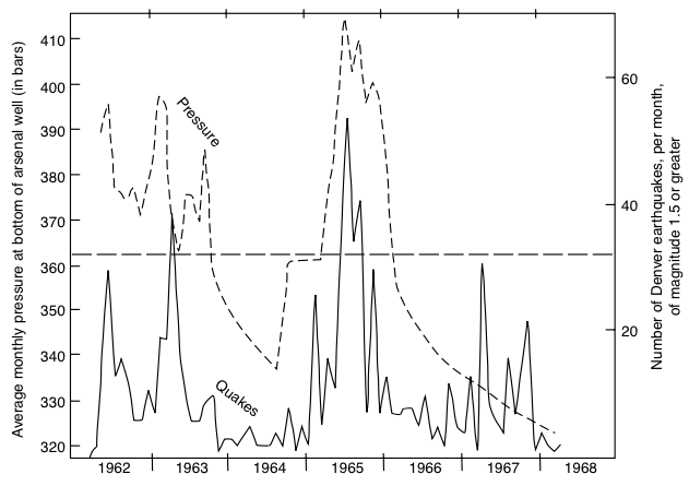
© Cambridge University Press Zoback, Reservoir Geomechanics (Fig. 4.22a, pp. 125)