Hydraulic Fracturing Modeling

Analytical Models

Analytical hydraulic fracture models use

• Fracture geometry assumptions
• Conservation of mass in fracture
• Elasticity theory for fracture opening
• Crack tip energetics

Perkins-Kern-Nordgren (PKN)

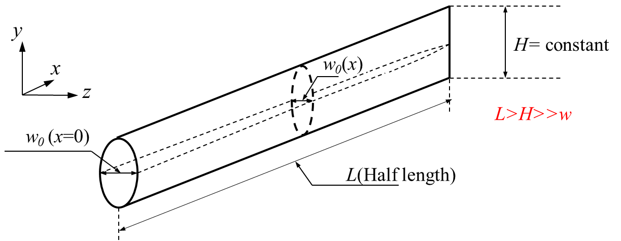
Schematic view of the PKN model Image Source

PKN Assumptions

• The formation toughness \(K_{Ic}\) can be neglected because the energy required to propagate in the fracture is significantly less than that required to allow fluid flow along the fracture
• The fluid is injected with a constant injection volumetric rate \(Q_0\) from a fixed line source at the center of the fracture into two wings
• The injected fluid is incompressible Newtonian laminar unidirectional flow characterized with viscosity \(\mu\) and the gravity effect is excluded
• Constant flow rate \(q\) along the fracture (No storage effect or fluid leakoff)
• The net pressure is zero at the tip

PKN Equations

\[\begin{align} L &= \frac{Q_0}{2 \pi C_L H} t^{\frac{1}{2}} \\ w_o &= \left(\frac{Q_0^2 \mu}{\pi^3 E^{\prime} C_L H}\right)^{\frac{1}{4}} t^{\frac{1}{8}} \\ p_o &= 2 \left( \frac{E^{\prime 3} Q_o^2 \mu}{\pi^3 C_L H^6}\right)^{\frac{1}{4}} t^{\frac{1}{8}} \end{align}\]

Kristianovich-Geertsma-de Klerk (KGD)

Image Source

Image Source

Figure 1: Schematic view of the KGD radial model and crack tip geometry

KGD Assumptions

• The formation is an infinite, homogeneous, isotropic, linear elastic medium characterized by Young’s modulus \(E\), Poisson’s ratio \(\nu\), and toughness \(K_{Ic}\).
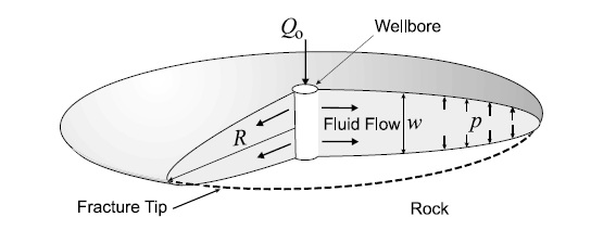
• The fracture is assumed to be radially symmetric and generated from a point-source at its center. The periphery of the fracture is circular (penny-shaped), as shown in Figure 1.
• The fracturing fluid is Newtonian with viscosity \(\mu\) . It is injected with a constant volumetric flow rate \(Q_o\), and its flow is laminar. Gravitational effects are not taken into account.
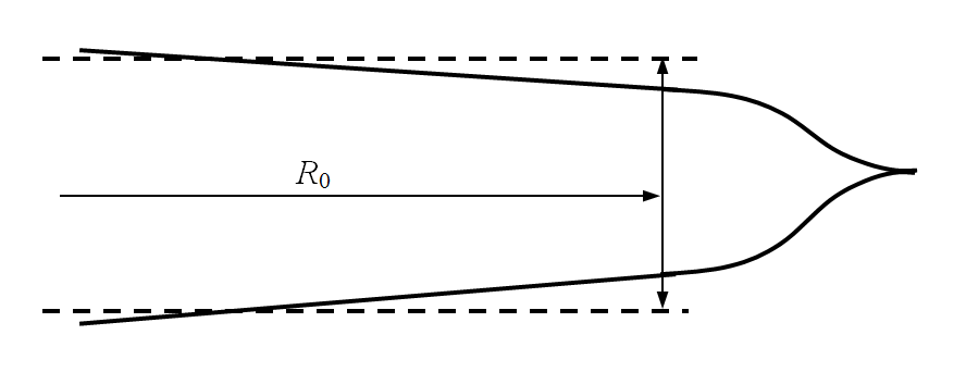
• The Barenblatt’s tip condition applies for the fracture.

KGD Equations (no leakoff)

\[\begin{align} R &= \left( \frac{3 E^{\prime} Q_0 t}{8 \sqrt{\pi} K_{Ic}}\right)^{0.4} \\ p_0 &= \frac{\sqrt{\pi} K_{Ic}}{2 \sqrt{R}} \\ w_0 &= \frac{8 p_0 R}{\pi E^{\prime}} \end{align}\]

Computational HF Models

• Displacement discontinuity method (DDM)
• Cohesive Zone Method
• Generalized FEM methods
• Phase-field fracture methods
• Peridynamics