Multi-Output Physics-Informed Neural Networks for Forward and Inverse PDE Problems with Uncertainties
August 18, 2023
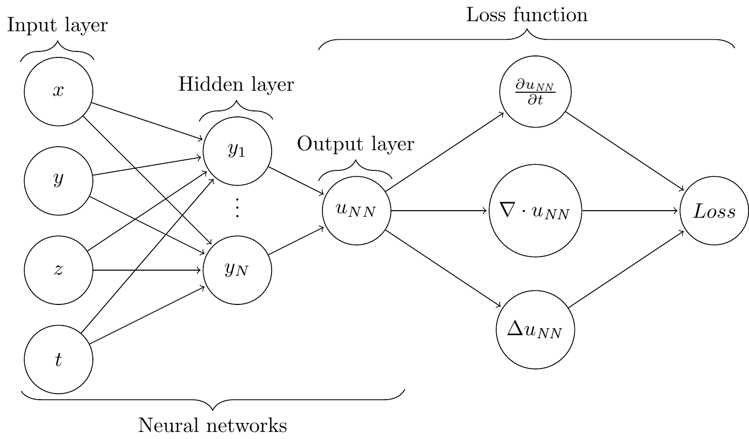
Generic PINN architecture
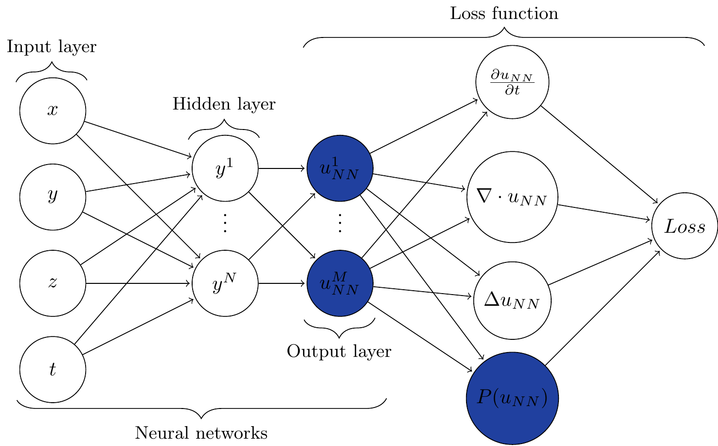
Multi-Output PINN
MO-PINN (M. Yang and Foster 2022)
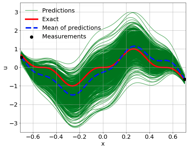
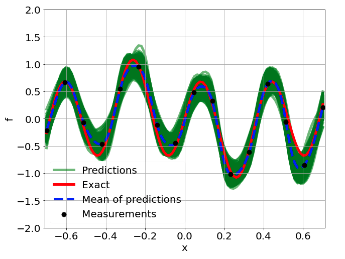
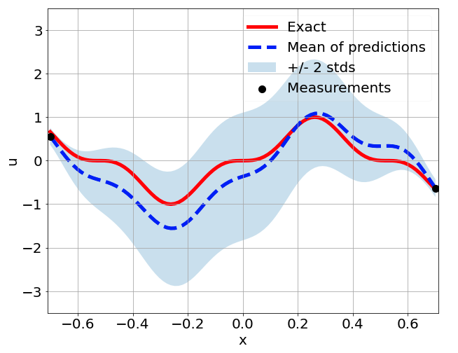
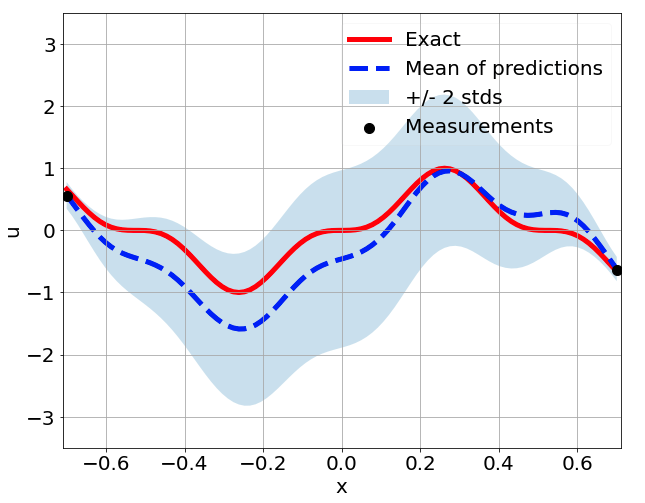
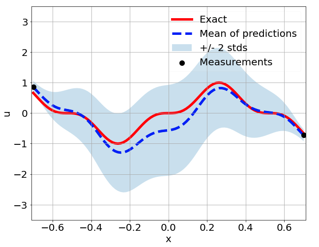
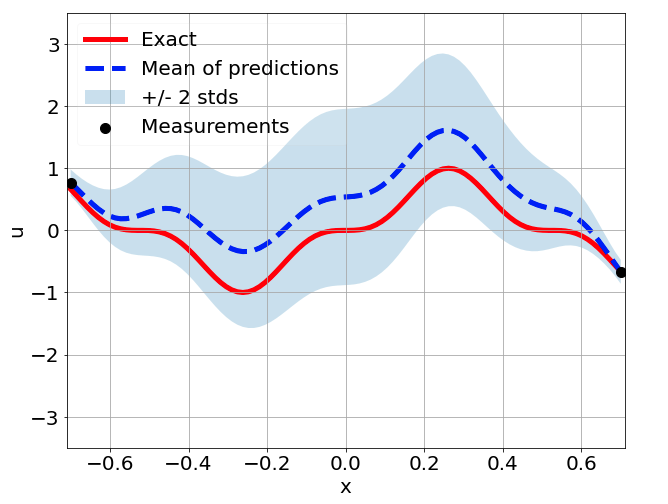
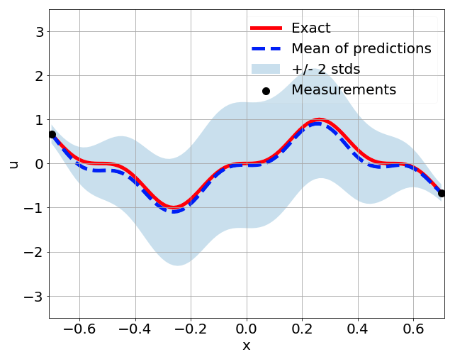
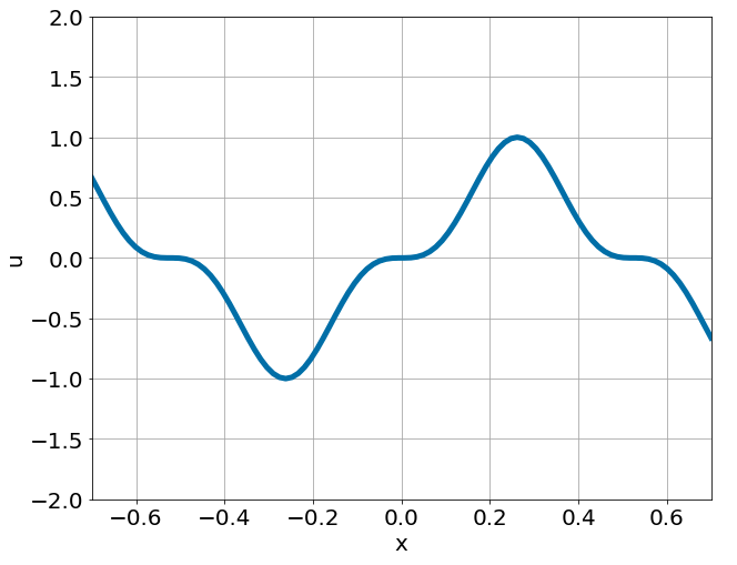
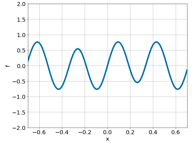
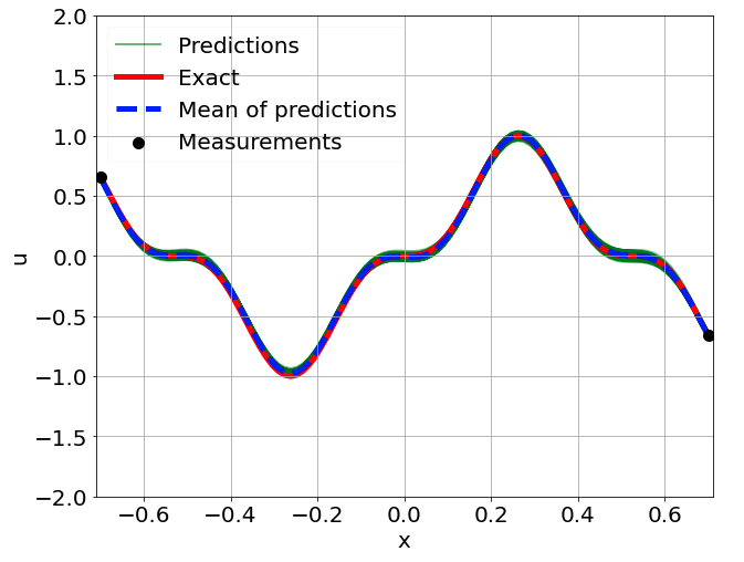
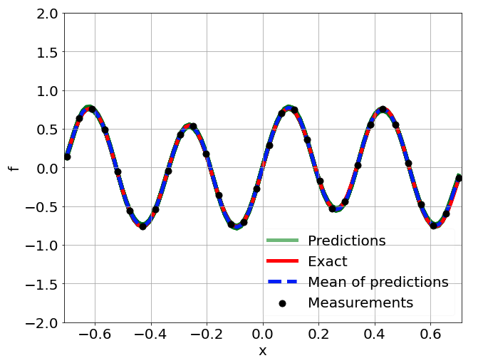
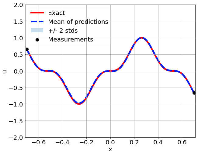
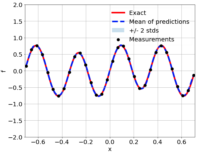
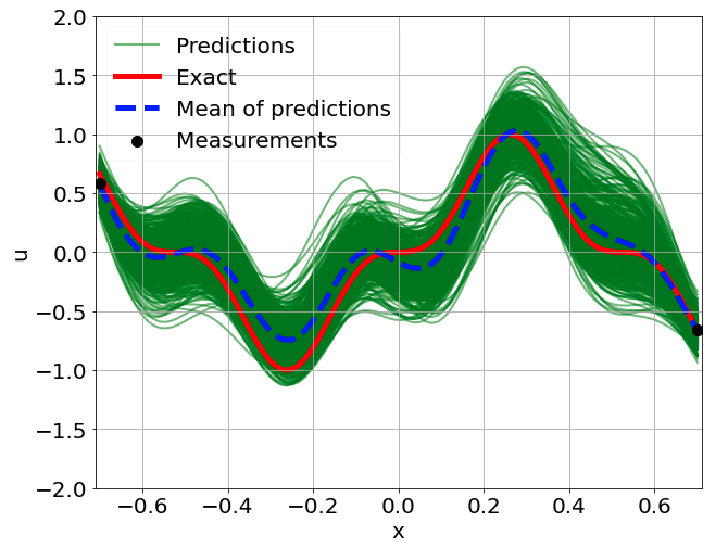
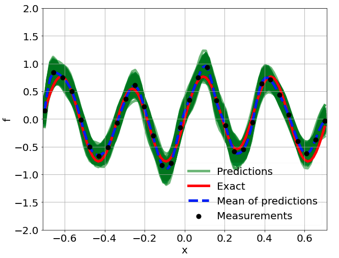
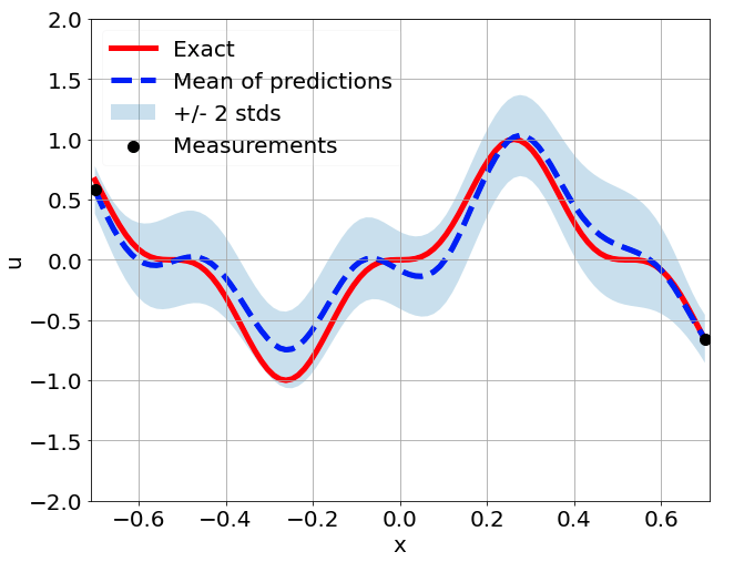
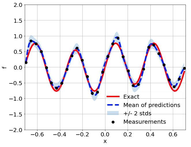
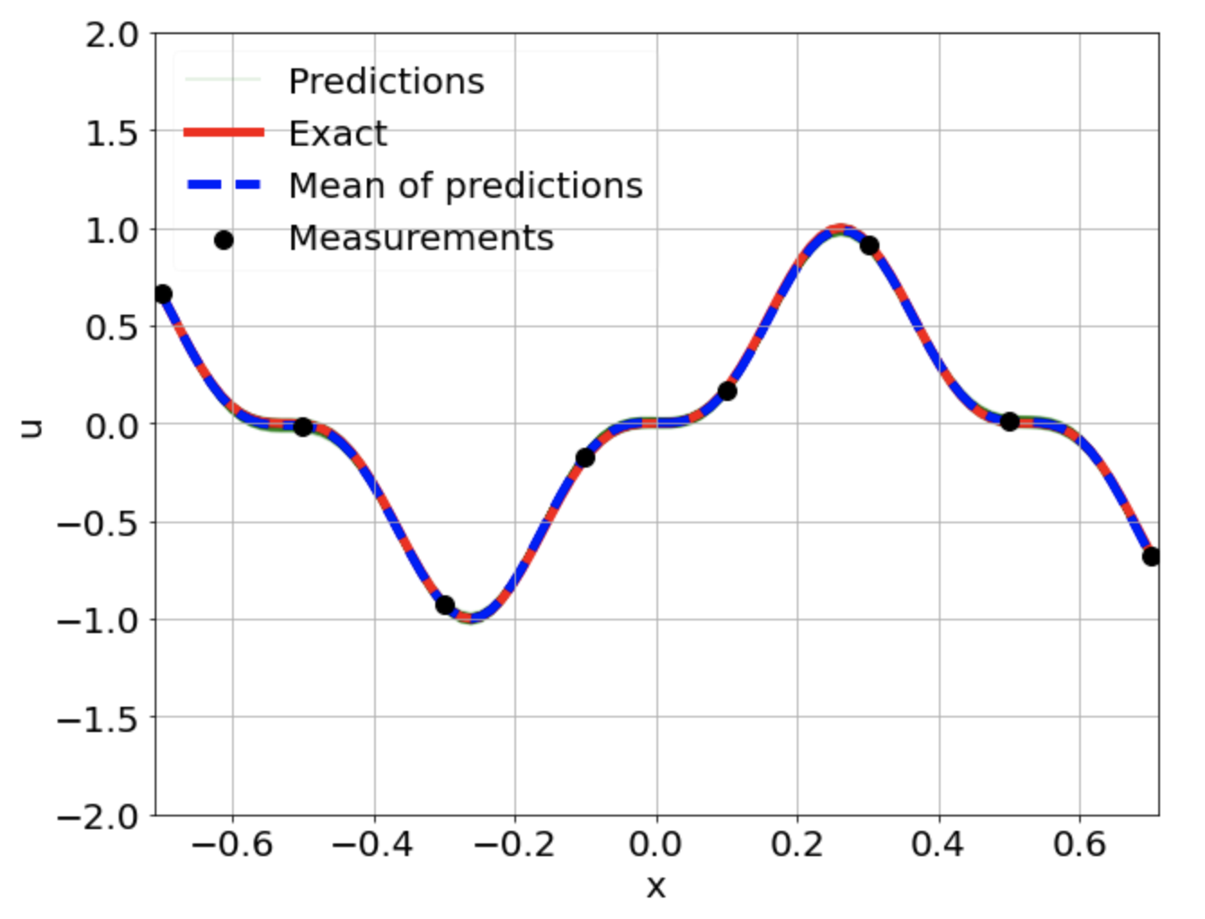
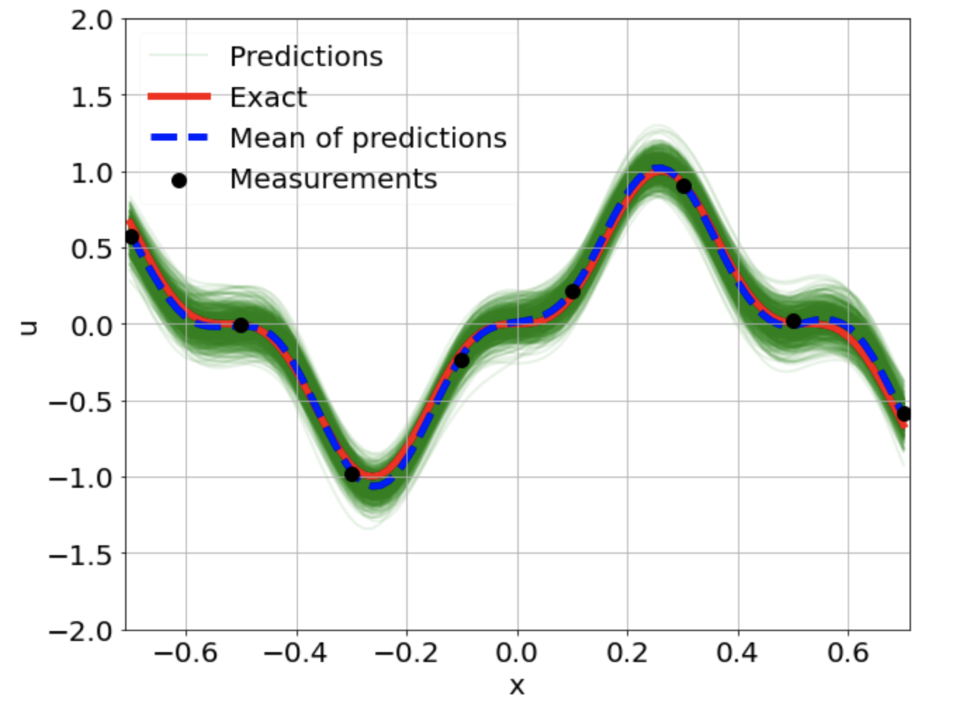
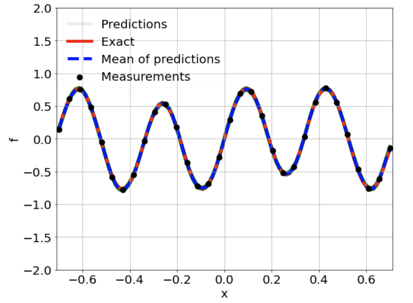
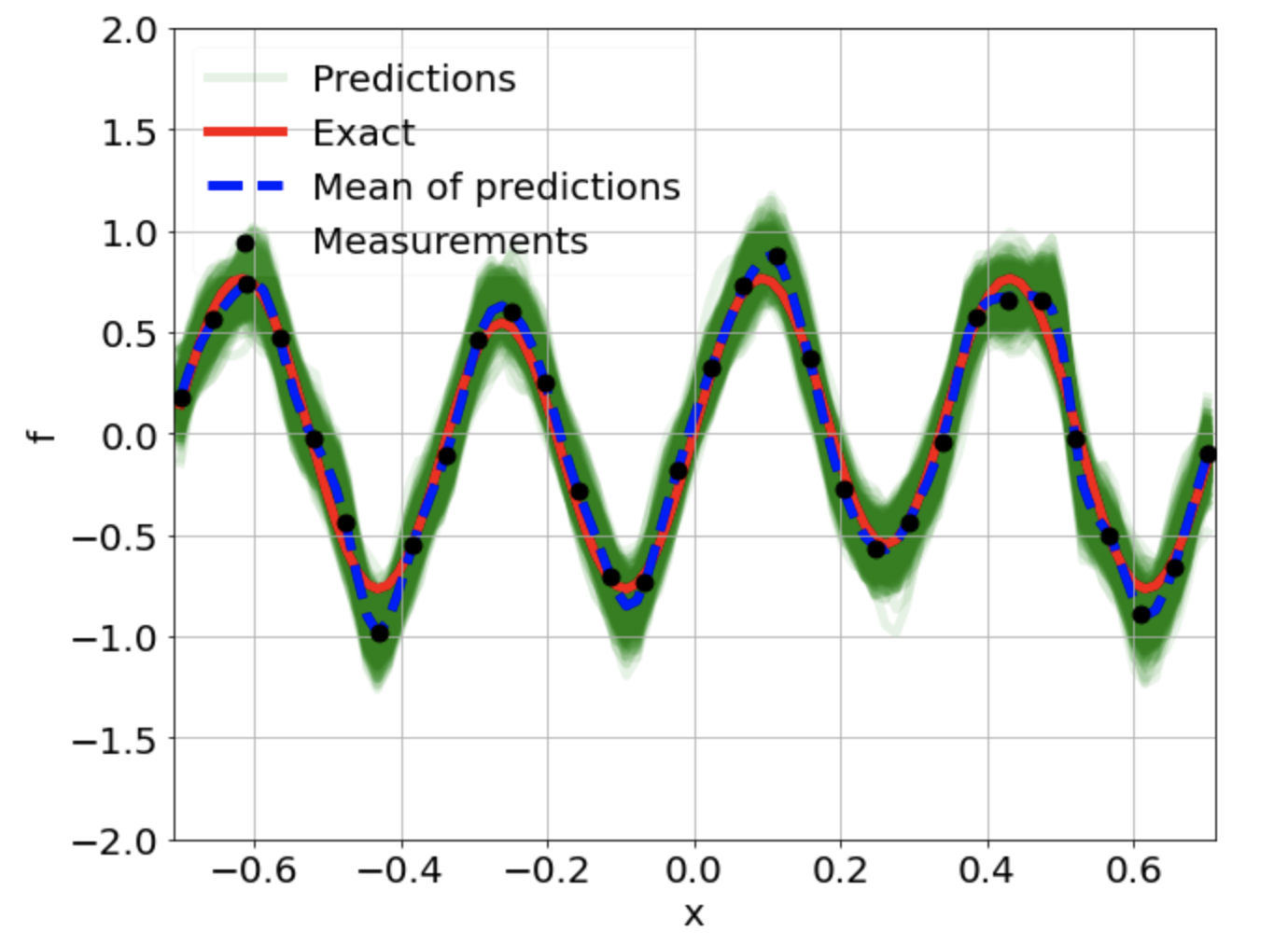
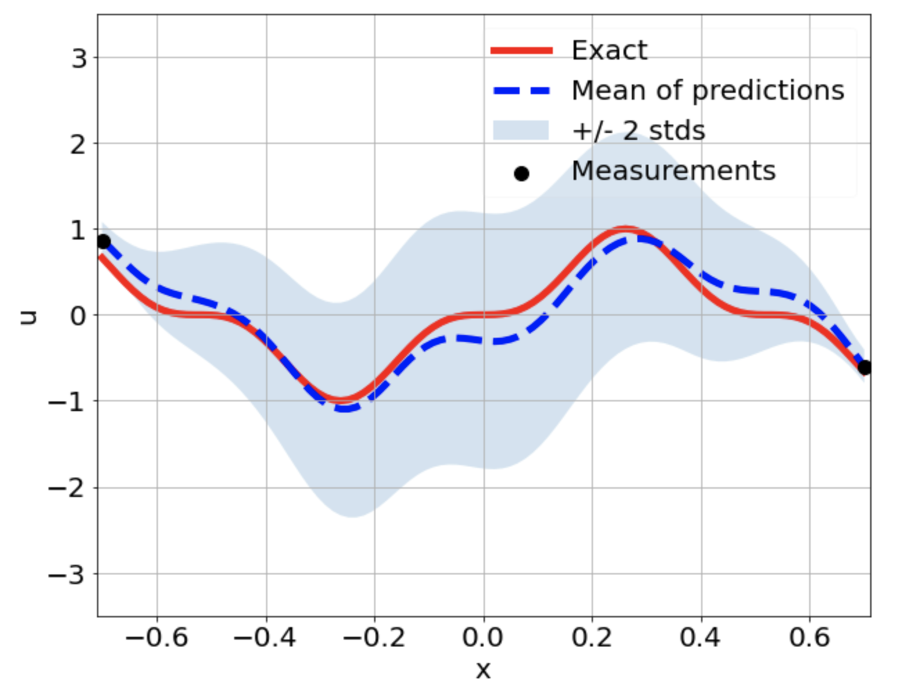
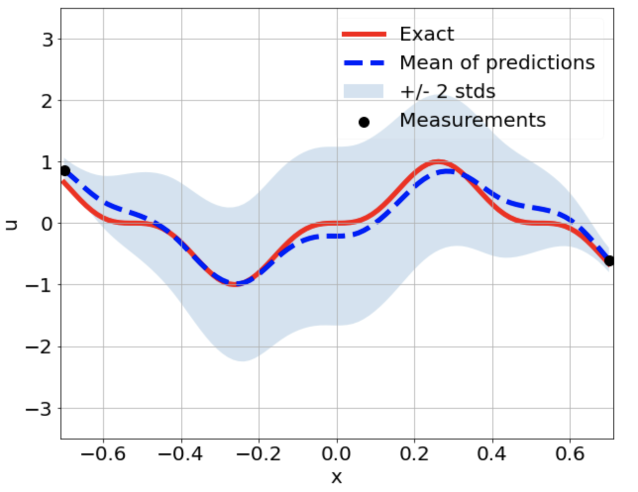
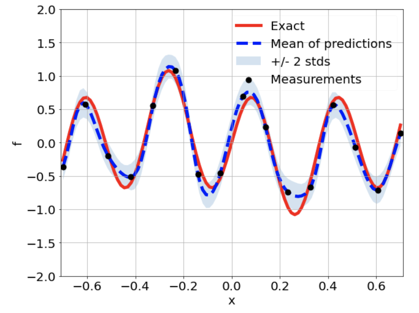
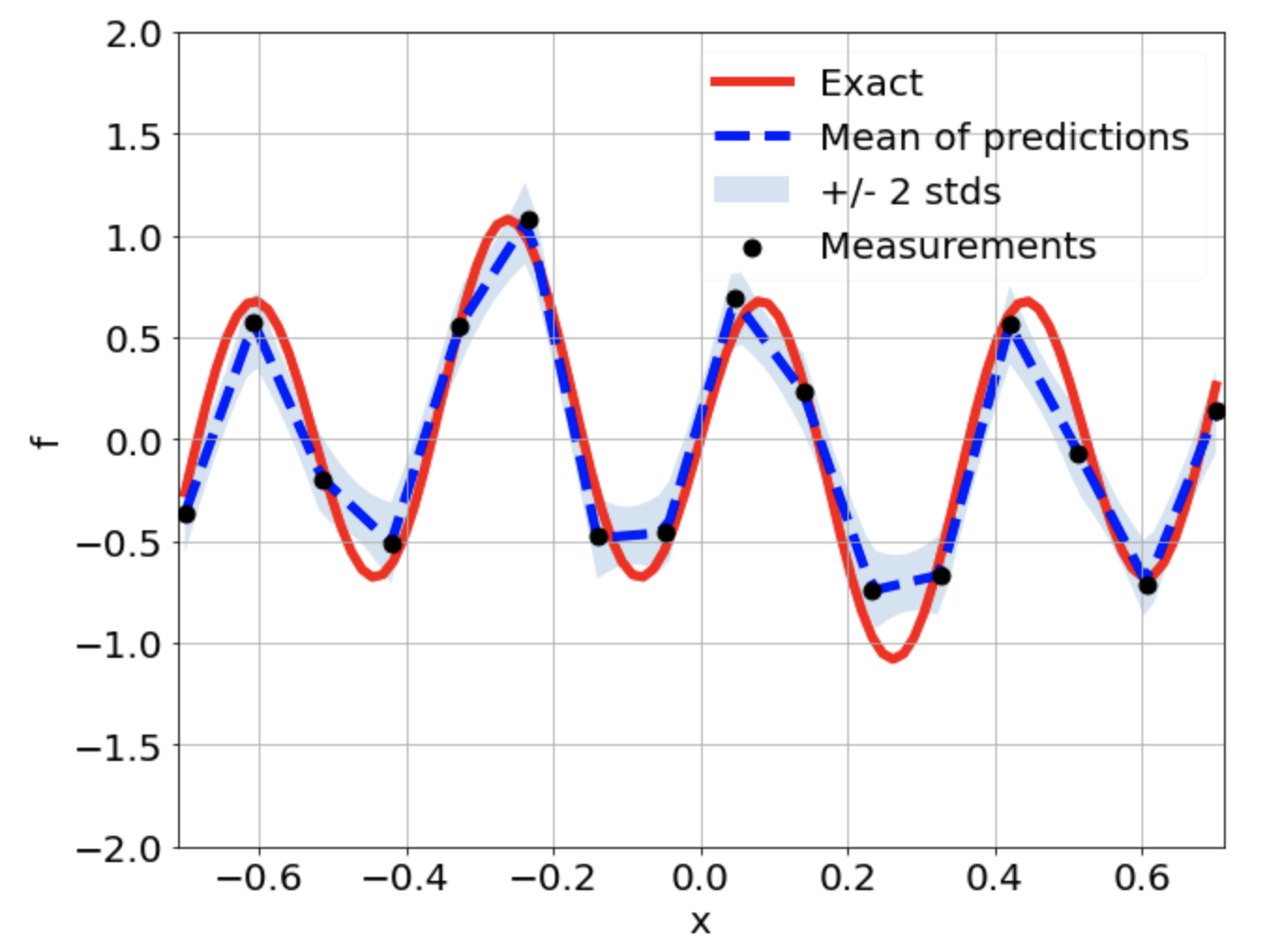
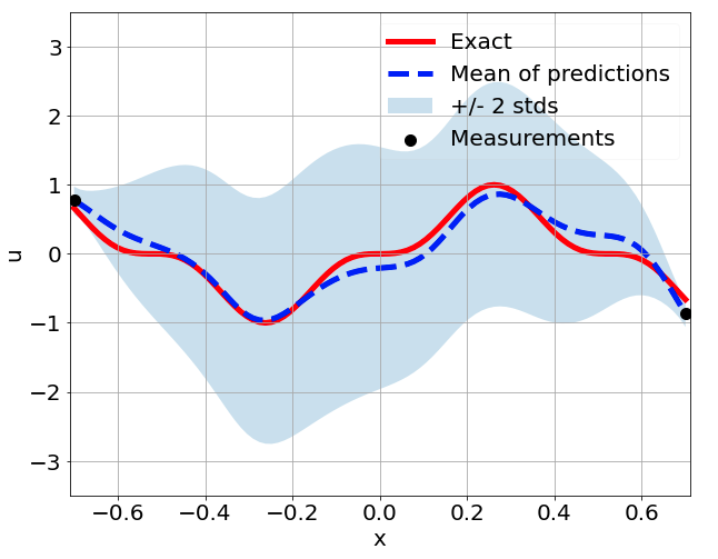
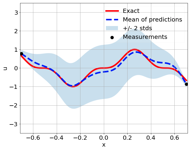
One-dimensional linear Poisson equation
\[ \begin{gathered} \lambda \frac{\partial^2 u}{\partial x^2} = f, \qquad x \in [-0.7, 0.7] \end{gathered} \] where \(\lambda = 0.01\) and \(u=\sin^3(6x)\)
Predictions w/ \(\sigma = 0.01\) noise on measurements
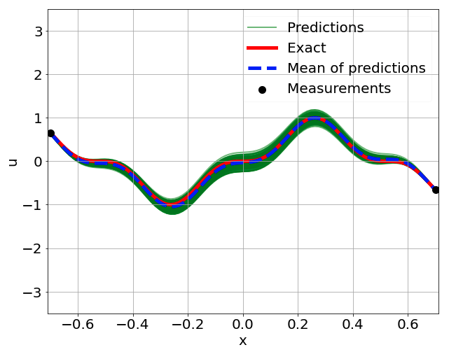
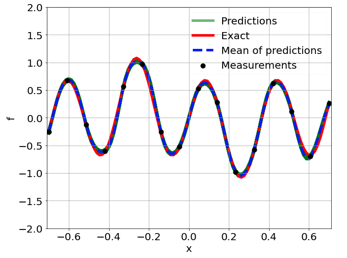
Predictions w/ \(\sigma = 0.1\) noise on measurements
Sensitivity to random network parameter initialization
\(\sigma = 0.1\) noise

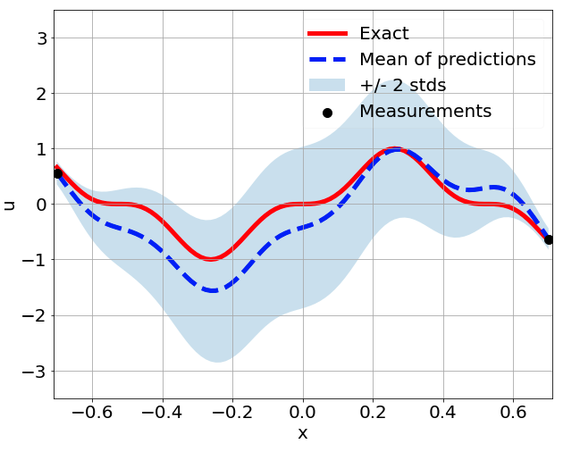
Sensitivity to measurement sampling
\(\sigma = 0.1\) noise
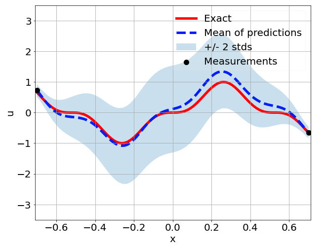
One-dimensional nonlinear Poisson equation
\[ \begin{gathered} \lambda \frac{\partial^2 u}{\partial x^2} + k \tanh(u) = f, \qquad x \in [-0.7, 0.7] \end{gathered} \] where \(\lambda = 0.01, k=0.7\) and \(u=\sin^3(6x)\)
Predictions w/ \(\sigma = 0.01\) noise on measurements
Predictions w/ \(\sigma = 0.1\) noise on measurements
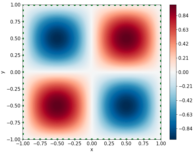
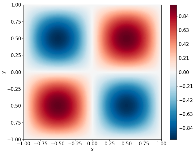
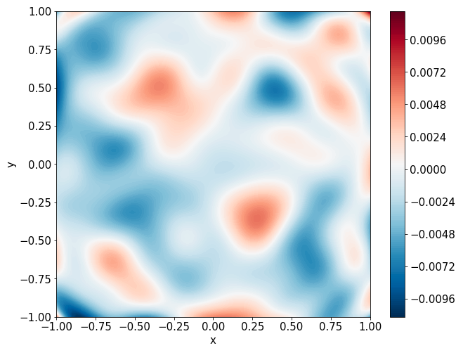
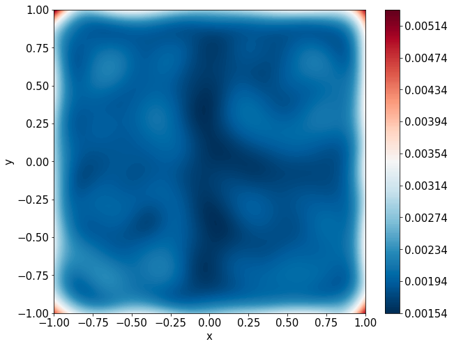
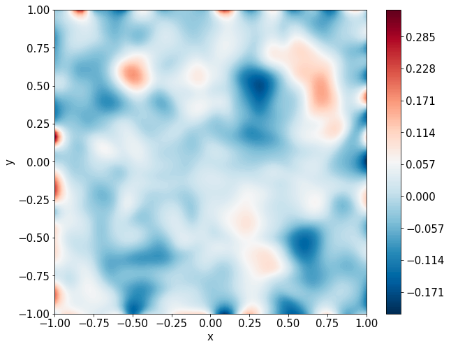
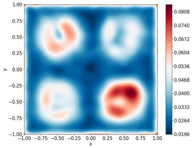
Two-dimensional nonlinear Allen-Cahn equation
\[ \begin{gathered} \lambda \left(\frac{\partial^2 u}{\partial x^2} + \frac{\partial^2 u}{\partial y^2}\right) + u\left(u^2 -1 \right) = f, \qquad x,y \in [-1, 1] \end{gathered} \] where \(\lambda = 0.01\) and \(u=\sin(\pi x)\sin(\pi y)\)

Predictions w/ \(\sigma = 0.01\) noise on measurements

Predictions w/ \(\sigma = 0.1\) noise on measurements
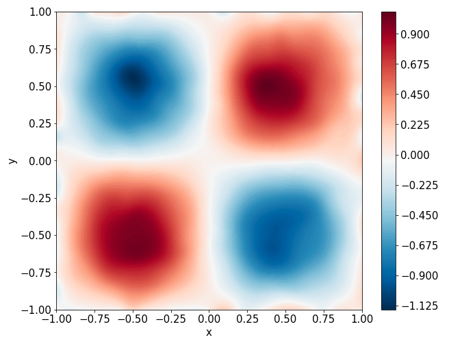

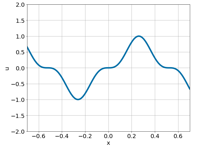
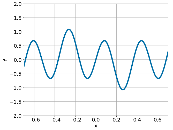
Predictions
\(u\) and \(f\)
Inverse Estimates
\(k_{exact} = 0.7\)
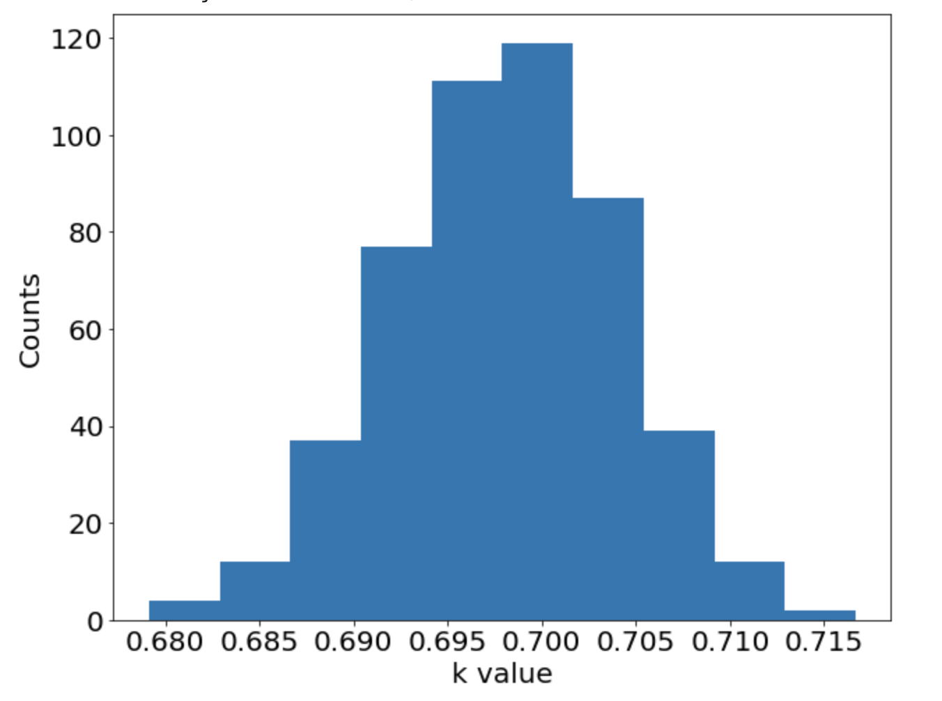
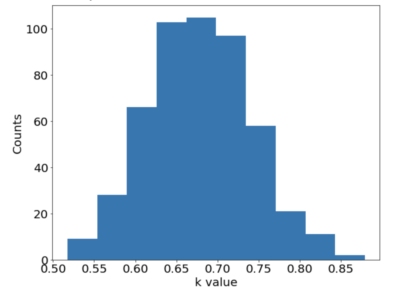
Sensitivity of \(k_{avg}\) w.r.t number of outputs
\(\sigma=0.1\) noise


Two-dimensional Allen-Cahn Equation
\[ \begin{gathered} \lambda \left(\frac{\partial^2 u}{\partial x^2} + \frac{\partial^2 u}{\partial y^2}\right) + u\left(u^2 -1 \right) = f, \qquad x,y \in [-1, 1] \end{gathered} \] where \(\lambda = 0.01\) and \(u=\sin(\pi x)\sin(\pi y)\)
\(k=[???, ???, ???, \dots, ???]\) with \(N\) entries corresponding to \(N\) outputs of the MO-PINN


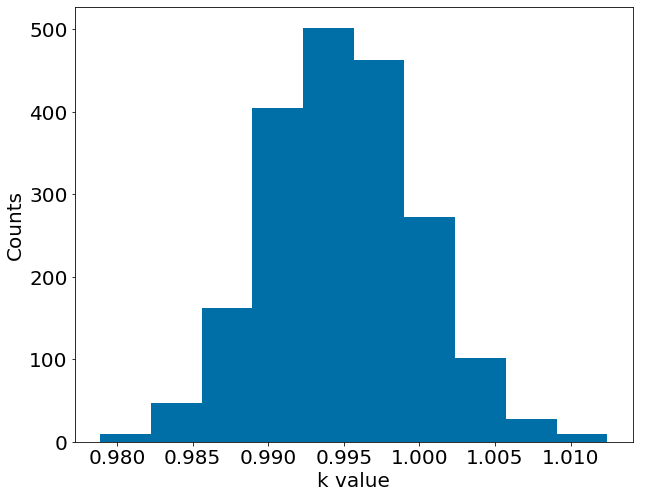
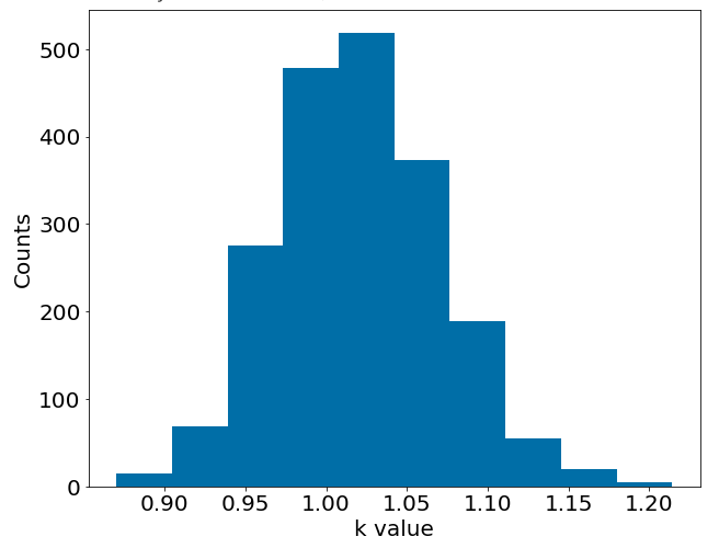
Inverse Estimates
\(k_{exact} = 1.0\)
Comparison to Monte Carlo FEM
One-dimensional linear Poisson equation
Comparison of distributions
MO-PINN vs. FEA Monte Carlo
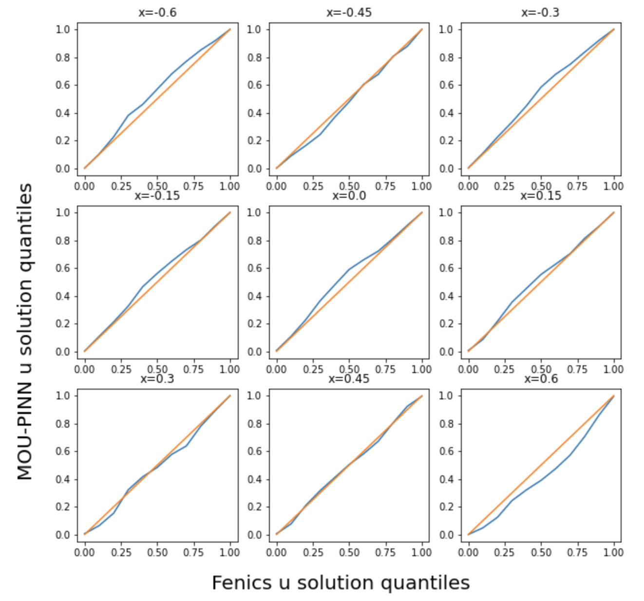
Quantile-quantile plot of \(u\) at 9 locations
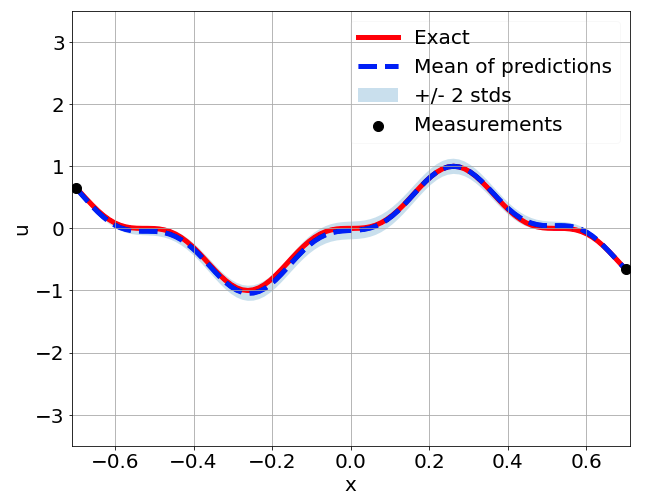
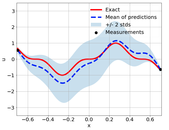
\(u\) predictions with only 5 measurements
Using mean and std to enhance learning

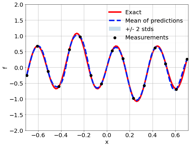
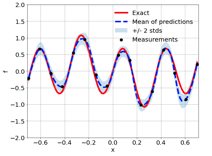
\(f\) predictions with only 5 measurements
Using mean and std to enhance learning


