Search
Pandas: Python Data Analysis Library

Pandas is a library for working with and manipulating tabular style data. In many ways you can think of it as a replacement for a spreadsheet only it's much more powerful. Whereas NumPy provides $N$-dimensional data structures, Pandas is best utilized on two-dimensional, labeled data. The fundamental data structures in Pandas are the Series and the Dataframe.

A Pandas Series contains a single column of data and an index. The index is a way to reference the rows of data in the Series. Common examples of an index would be simply a monotonically increasing set of integers, or time/date stamps for time series data.

A Pandas DataFrame can be thought of being created by combining more than one Series that share a common index. So a table with multiple column labels and common index would be an example of a DataFrame. The description of these data structures will be made clear through examples in the sequel.

Similarly to the way we import NumPy, it's idiomatic Python to import Pandas as

import pandas as pd
import numpy as np
import pandas as pd

Loading Data

Pandas offers some of the best utilities available for reading/parsing data from text files. The function read_csv has numerous options for managing header/footer lines in files, parsing dates, selecting specific columns, etc in comma separated value (CSV) files. The default index for the Dataframe is set to a set of monotonically increasing integers unless otherwise specified with the keyword argument index_col.

There are similar functions for reading Microsoft Excel spreadsheets (read_excel) and fixed width formatted text (read_fwf).

The file '200wells.csv' contains a dataset with X and Y coordinates, facies 1 and 2 (1 is sandstone and 2 interbedded sand and mudstone), porosity , permeability (mD) and acoustic impedance ($\mbox{kg} / (\mbox{m}^2 \cdot \mbox{s} \cdot 10^6)$).

The head() member function for DataFrames displays the first 5 rows of the DataFrame. Optionally, you can specify an argument (e.g. head(n=10) to display more/less rows

df = pd.read_csv('datasets/200wells.csv'); df.head()
Unnamed: 0 X Y facies_threshold_0.3 porosity permeability acoustic_impedance
0 0 565 1485 1 0.1184 6.170 2.009
1 1 2585 1185 1 0.1566 6.275 2.864
2 2 2065 2865 2 0.1920 92.297 3.524
3 3 3575 2655 1 0.1621 9.048 2.157
4 4 1835 35 1 0.1766 7.123 3.979

Summary Statistics

The DataFrame member function describe provides useful summary statistics such as the total number of samples, mean, standard deviations, min/max, and quartiles for each column of the DataFrame.

df.describe()
Unnamed: 0 X Y facies_threshold_0.3 porosity permeability acoustic_impedance
count 200.000000 200.000000 200.00000 200.000000 200.000000 200.000000 200.000000
mean 99.500000 2053.400000 1876.15000 1.330000 0.149300 25.287462 3.000435
std 57.879185 1113.524641 1137.58016 0.471393 0.032948 64.470135 0.592201
min 0.000000 25.000000 35.00000 1.000000 0.050000 0.015820 2.009000
25% 49.750000 1112.500000 920.00000 1.000000 0.132175 1.366750 2.483250
50% 99.500000 2160.000000 1855.00000 1.000000 0.150150 4.825500 2.964500
75% 149.250000 2915.000000 2782.50000 2.000000 0.174200 14.597000 3.527000
max 199.000000 3955.000000 3995.00000 2.000000 0.223200 463.641000 3.984000

Indexing and Selecting Data

We can access parts of the DataFrame by their labels or their numerical indices. The most basic and useful operation is to select an entire column of data by it's label.

df[['porosity']].head()
porosity
0 0.1184
1 0.1566
2 0.1920
3 0.1621
4 0.1766

Multiple columns can be selected by passing in a list of labels.

df[['porosity', 'permeability']].head()
porosity permeability
0 0.1184 6.170
1 0.1566 6.275
2 0.1920 92.297
3 0.1621 9.048
4 0.1766 7.123

Label based selection

The member function loc can be used to select both rows and columns of data by their labels. The index is interpreted as the row label.

df.loc[1:2, ['porosity', 'permeability']]
porosity permeability
1 0.1566 6.275
2 0.1920 92.297

loc support NumPy-style slicing notation to select sequences of labels.

df.loc[1:2, 'porosity':'acoustic_impedance']
porosity permeability acoustic_impedance
1 0.1566 6.275 2.864
2 0.1920 92.297 3.524

Index based selection

The member function iloc can be used to select both rows and columns of data by their integer index. iloc supports Python-list style slicing.

df.iloc[1:3, 3:5]
facies_threshold_0.3 porosity
1 1 0.1566
2 2 0.1920

Get data as NumPy array

We can get the underlying data in a Series/DataFrame as a NumPy array with the values attribute.

df['porosity'].values
array([0.1184 , 0.1566 , 0.192  , 0.1621 , 0.1766 , 0.1239 , 0.179  ,
       0.1914 , 0.1763 , 0.1674 , 0.1369 , 0.1095 , 0.1677 , 0.1817 ,
       0.119  , 0.1774 , 0.1418 , 0.1296 , 0.1325 , 0.1729 , 0.08494,
       0.188  , 0.1147 , 0.1795 , 0.1981 , 0.1258 , 0.215  , 0.1781 ,
       0.1428 , 0.1495 , 0.1435 , 0.1026 , 0.1772 , 0.19   , 0.1597 ,
       0.1453 , 0.1653 , 0.176  , 0.2232 , 0.1336 , 0.1819 , 0.1591 ,
       0.1328 , 0.1517 , 0.1061 , 0.08187, 0.1682 , 0.1367 , 0.1628 ,
       0.1305 , 0.1097 , 0.2062 , 0.168  , 0.1663 , 0.1231 , 0.1965 ,
       0.1292 , 0.1347 , 0.1481 , 0.1523 , 0.1388 , 0.1574 , 0.1769 ,
       0.1982 , 0.161  , 0.1584 , 0.1594 , 0.1146 , 0.1367 , 0.1742 ,
       0.1585 , 0.1065 , 0.181  , 0.1372 , 0.1384 , 0.0991 , 0.137  ,
       0.1957 , 0.1032 , 0.1973 , 0.1336 , 0.1792 , 0.152  , 0.08245,
       0.1505 , 0.0938 , 0.1563 , 0.1277 , 0.141  , 0.1712 , 0.1428 ,
       0.07338, 0.1595 , 0.1079 , 0.1191 , 0.132  , 0.1394 , 0.2154 ,
       0.1428 , 0.1416 , 0.1658 , 0.187  , 0.1796 , 0.177  , 0.1714 ,
       0.1438 , 0.186  , 0.0964 , 0.1455 , 0.1322 , 0.06726, 0.1162 ,
       0.1021 , 0.1396 , 0.1139 , 0.1576 , 0.1417 , 0.2159 , 0.1352 ,
       0.0964 , 0.1853 , 0.1898 , 0.1785 , 0.1648 , 0.1367 , 0.1644 ,
       0.1376 , 0.1974 , 0.1498 , 0.1524 , 0.1579 , 0.147  , 0.1105 ,
       0.1825 , 0.1227 , 0.1414 , 0.1347 , 0.165  , 0.2019 , 0.1487 ,
       0.1784 , 0.0784 , 0.1061 , 0.1491 , 0.0915 , 0.1677 , 0.1811 ,
       0.1377 , 0.2158 , 0.1356 , 0.1062 , 0.132  , 0.05   , 0.08678,
       0.1474 , 0.164  , 0.15   , 0.1606 , 0.1478 , 0.1645 , 0.1415 ,
       0.1821 , 0.1319 , 0.08012, 0.2158 , 0.177  , 0.08209, 0.1254 ,
       0.1611 , 0.1916 , 0.1742 , 0.2063 , 0.122  , 0.1541 , 0.1435 ,
       0.1505 , 0.192  , 0.1104 , 0.1717 , 0.1394 , 0.1503 , 0.18   ,
       0.164  , 0.1808 , 0.1577 , 0.1211 , 0.1523 , 0.1467 , 0.1591 ,
       0.1367 , 0.192  , 0.1359 , 0.1513 , 0.1473 , 0.1377 , 0.1634 ,
       0.1548 , 0.1321 , 0.06092, 0.1505 ])

DataFrame Transformations

There are several member functions that allow for transformations of the DataFrame labels, adding/removing columns, etc.

To rename DataFrame column labels, we pass a Python dictionary where the keywords are the current labels and the values are the new labels. For example,

The use of the keyword argument inplace = True has an equivalent outcome as writing

df = df.rename(...
df.rename(columns={'facies_threshold_0.3': 'facies', 
                   'permeability': 'perm', 
                   'acoustic_impedance': 'ai'}, inplace = True)
df.head()
Unnamed: 0 X Y facies porosity perm ai
0 0 565 1485 1 0.1184 6.170 2.009
1 1 2585 1185 1 0.1566 6.275 2.864
2 2 2065 2865 2 0.1920 92.297 3.524
3 3 3575 2655 1 0.1621 9.048 2.157
4 4 1835 35 1 0.1766 7.123 3.979

Adding a New Column

Pandas DataFrames share a lot of the same syntax with Python dictionaries including accessing columns by label (i.e. keyword) and adding entries. The example below shows how to add a new column with the label 'zero'.

df['zero'] = np.zeros(len(df)) 
df.head()
Unnamed: 0 X Y facies porosity perm ai zero
0 0 565 1485 1 0.1184 6.170 2.009 0.0
1 1 2585 1185 1 0.1566 6.275 2.864 0.0
2 2 2065 2865 2 0.1920 92.297 3.524 0.0
3 3 3575 2655 1 0.1621 9.048 2.157 0.0
4 4 1835 35 1 0.1766 7.123 3.979 0.0

Removing Columns

We can remove unwanted columns with the drop member function. The argument inplace = True modifies the existing DataFrame in place in memory, i.e. 'zero' will no longer be accessible in any way in the DataFrame.

The argument axis = 1 refers to columns, the default is axis = 0 in which case the positional argument would be expected to be an index label.

df.drop('zero', axis=1, inplace=True)
df.head()
Unnamed: 0 X Y facies porosity perm ai
0 0 565 1485 1 0.1184 6.170 2.009
1 1 2585 1185 1 0.1566 6.275 2.864
2 2 2065 2865 2 0.1920 92.297 3.524
3 3 3575 2655 1 0.1621 9.048 2.157
4 4 1835 35 1 0.1766 7.123 3.979

Removing Rows

We can remove the row indexed by 1 as follows.

Notice we can stack member function commands, i.e. the drop function is immediately followed by head to display the DataFrame with row index 1 removed.

df.drop(1).head()
Unnamed: 0 X Y facies porosity perm ai
0 0 565 1485 1 0.1184 6.170 2.009
2 2 2065 2865 2 0.1920 92.297 3.524
3 3 3575 2655 1 0.1621 9.048 2.157
4 4 1835 35 1 0.1766 7.123 3.979
5 5 3375 2525 1 0.1239 1.468 2.337

Because the argument inplace = True was not given, the orginal DataFrame is unchanged.

df.head()
Unnamed: 0 X Y facies porosity perm ai
0 0 565 1485 1 0.1184 6.170 2.009
1 1 2585 1185 1 0.1566 6.275 2.864
2 2 2065 2865 2 0.1920 92.297 3.524
3 3 3575 2655 1 0.1621 9.048 2.157
4 4 1835 35 1 0.1766 7.123 3.979

Sorting

We can sort the DataFrame in either ascending or desending order by any column label.

df.sort_values('porosity', ascending=False, inplace=True)
df.head(n=13)
Unnamed: 0 X Y facies porosity perm ai
38 38 3505 1525 2 0.2232 174.654 3.344
117 117 2665 3205 2 0.2159 273.980 2.551
164 164 2455 2885 2 0.2158 9.592 2.773
148 148 1975 2745 2 0.2158 361.704 3.839
97 97 1855 3025 2 0.2154 463.641 3.091
26 26 1785 3145 2 0.2150 201.363 2.877
171 171 3735 2585 1 0.2063 30.258 2.100
51 51 1655 2985 2 0.2062 17.585 3.444
138 138 1855 3095 2 0.2019 257.990 2.886
63 63 845 3915 1 0.1982 410.570 2.781
24 24 2625 3185 1 0.1981 124.222 2.451
127 127 1615 2285 2 0.1974 159.567 3.167
79 79 1265 3105 2 0.1973 114.044 2.750

Reseting Indices

In the previous example, the resulting indices are now out of order after the sorting operation. This can be fixed, if desired, with the reset_index member function.

The reindexing operation could have been accomplished during the sort operation by passing the argument ingnore_index = True.

df.reset_index(inplace=True, drop=True)
df.head(n = 13)
Unnamed: 0 X Y facies porosity perm ai
0 38 3505 1525 2 0.2232 174.654 3.344
1 117 2665 3205 2 0.2159 273.980 2.551
2 164 2455 2885 2 0.2158 9.592 2.773
3 148 1975 2745 2 0.2158 361.704 3.839
4 97 1855 3025 2 0.2154 463.641 3.091
5 26 1785 3145 2 0.2150 201.363 2.877
6 171 3735 2585 1 0.2063 30.258 2.100
7 51 1655 2985 2 0.2062 17.585 3.444
8 138 1855 3095 2 0.2019 257.990 2.886
9 63 845 3915 1 0.1982 410.570 2.781
10 24 2625 3185 1 0.1981 124.222 2.451
11 127 1615 2285 2 0.1974 159.567 3.167
12 79 1265 3105 2 0.1973 114.044 2.750

Feature Engineering

In the field of data science, DataFrame column labels are often referred to as features. Feature engineering is the process of creating new features and/or transforming features for further analysis. In the example below, we create two new features through manipulations of existing features.

Mathematical operations can be performed directly on the DataFrame columns that are accessed by their labels.

df['% porosity'] = df['porosity'] * 100
df['perm-por ratio'] = df['perm'] / df['porosity']          
df.head()
Unnamed: 0 X Y facies porosity perm ai % porosity perm-por ratio
0 38 3505 1525 2 0.2232 174.654 3.344 22.32 782.500000
1 117 2665 3205 2 0.2159 273.980 2.551 21.59 1269.013432
2 164 2455 2885 2 0.2158 9.592 2.773 21.58 44.448563
3 148 1975 2745 2 0.2158 361.704 3.839 21.58 1676.107507
4 97 1855 3025 2 0.2154 463.641 3.091 21.54 2152.465181

Assigning Conditional Categories

We can also use conditional statements when assigning values to a new feature. For example, we could have a categorical porosity measure for high and low porosity, called 'porosity type'.

Most NumPy functions such as where will work directly on Pandas DataFrame columns.

df['porosity type'] = np.where(df['porosity'] > 0.12, 'high', 'low')
df[df['porosity type'] == 'high'].head(n=3)
Unnamed: 0 X Y facies porosity perm ai % porosity perm-por ratio porosity type
0 38 3505 1525 2 0.2232 174.654 3.344 22.32 782.500000 high
1 117 2665 3205 2 0.2159 273.980 2.551 21.59 1269.013432 high
2 164 2455 2885 2 0.2158 9.592 2.773 21.58 44.448563 high
df[df['porosity type'] == 'low'].head(n=3)
Unnamed: 0 X Y facies porosity perm ai % porosity perm-por ratio porosity type
165 94 1365 2715 1 0.1191 0.2666 2.788 11.91 2.238455 low
166 14 2765 925 1 0.1190 0.7731 2.323 11.90 6.496639 low
167 0 565 1485 1 0.1184 6.1700 2.009 11.84 52.111486 low

Feature Truncation

Here's an example where we use a conditional statement to assign a very low permeability value (0.0001 mD) for all porosity values below a threshold. Of course, this is for demonstration, in practice a much lower porosity threshold would likely be applied.

df['perm cutoff'] = np.where(df['porosity'] > 0.12, df['perm'], 0.0001) 
df.head(n=3)
Unnamed: 0 X Y facies porosity perm ai % porosity perm-por ratio porosity type perm cutoff
0 38 3505 1525 2 0.2232 174.654 3.344 22.32 782.500000 high 174.654
1 117 2665 3205 2 0.2159 273.980 2.551 21.59 1269.013432 high 273.980
2 164 2455 2885 2 0.2158 9.592 2.773 21.58 44.448563 high 9.592
df[df['perm cutoff'] == 0.0001].head(n=3)
Unnamed: 0 X Y facies porosity perm ai % porosity perm-por ratio porosity type perm cutoff
165 94 1365 2715 1 0.1191 0.2666 2.788 11.91 2.238455 low 0.0001
166 14 2765 925 1 0.1190 0.7731 2.323 11.90 6.496639 low 0.0001
167 0 565 1485 1 0.1184 6.1700 2.009 11.84 52.111486 low 0.0001

Applying functions to Series/DataFrame

We can apply any function that we can define in Python to entries of a Series or DataFrame. First we define a function. This function returns the Kozeny-Carmen relationship to predict permeability from porosity ϕ, for values of ϕ greater that $0.12$, otherwise it returns $0.0001$. The proportionality constant $m$ is given as an additional keyword argument.

def kozeny_carmen_with_threshold(ϕ, m=5):
    
    if ϕ > 0.12:
        return m * ϕ ** 3 / (1 - ϕ) ** 2
    else:
        return 0.0001

Using the apply member function we can transform the 'porosity' column into permeability via the kozeny_carmen_with_threshold function above.

df['kozeny carmen'] = df['porosity'].apply(kozeny_carmen_with_threshold, m=10)
df
Unnamed: 0 X Y facies porosity perm ai % porosity perm-por ratio porosity type perm cutoff kozeny carmen
0 38 3505 1525 2 0.22320 174.65400 3.344 22.320 782.500000 high 174.6540 0.184274
1 117 2665 3205 2 0.21590 273.98000 2.551 21.590 1269.013432 high 273.9800 0.163687
2 164 2455 2885 2 0.21580 9.59200 2.773 21.580 44.448563 high 9.5920 0.163418
3 148 1975 2745 2 0.21580 361.70400 3.839 21.580 1676.107507 high 361.7040 0.163418
4 97 1855 3025 2 0.21540 463.64100 3.091 21.540 2152.465181 high 463.6410 0.162346
... ... ... ... ... ... ... ... ... ... ... ... ...
195 141 1745 255 2 0.07840 1.01500 3.949 7.840 12.946429 low 0.0001 0.000100
196 91 3835 1095 1 0.07338 0.02198 3.775 7.338 0.299537 low 0.0001 0.000100
197 110 2365 355 1 0.06726 0.15170 3.833 6.726 2.255427 low 0.0001 0.000100
198 198 3795 535 1 0.06092 0.01582 3.907 6.092 0.259685 low 0.0001 0.000100
199 152 3745 115 1 0.05000 0.01653 3.527 5.000 0.330600 low 0.0001 0.000100

200 rows × 12 columns

Missing Features

It's very common in data analysis to have missing and/or invalid values in our our DataFrames. Pandas offers several built in methods to identify and deal with missing Data.

First, let's create a missing data point in the 'porosity' column of df.

The at member function allows for fast selection of a single row/label position within a Series/DataFrame.

df.at[1, 'porosity'] = None
df.head(n = 3)
Unnamed: 0 X Y facies porosity perm ai % porosity perm-por ratio porosity type perm cutoff kozeny carmen
0 38 3505 1525 2 0.2232 174.654 3.344 22.32 782.500000 high 174.654 0.184274
1 117 2665 3205 2 NaN 273.980 2.551 21.59 1269.013432 high 273.980 0.163687
2 164 2455 2885 2 0.2158 9.592 2.773 21.58 44.448563 high 9.592 0.163418

The isnull member function returns a boolean array that identifies rows with missing values.

df[df['porosity'].isnull()]
Unnamed: 0 X Y facies porosity perm ai % porosity perm-por ratio porosity type perm cutoff kozeny carmen
1 117 2665 3205 2 NaN 273.98 2.551 21.59 1269.013432 high 273.98 0.163687

Dropping missing rows

The dropna member function allows us to remove missing rows from the DataFrame.

df.dropna(inplace=True)
df.head(n = 3)
Unnamed: 0 X Y facies porosity perm ai % porosity perm-por ratio porosity type perm cutoff kozeny carmen
0 38 3505 1525 2 0.2232 174.654 3.344 22.32 782.500000 high 174.654 0.184274
2 164 2455 2885 2 0.2158 9.592 2.773 21.58 44.448563 high 9.592 0.163418
3 148 1975 2745 2 0.2158 361.704 3.839 21.58 1676.107507 high 361.704 0.163418

Creating New DataFrames

Up to now, we've utilized a DataFrame that was created by reading in the data from a CSV file. We can also create DataFrames from scratch. First we'll create a couple of NumPy arrays with representative data for demonstration.

porosity = np.random.random_sample(100) * 0.2
permeability = 10 * porosity ** 3 / (1 - porosity) ** 2 

Create a Python dictionary where the keywords are the desired DataFrame labels and the values are the associated data.

df_dict = {'porosity': porosity, 'permeability': permeability}

Pass the dictionary as an argument to pd.Dataframe to create the DataFrame

df_new = pd.DataFrame(df_dict)
df_new.sort_values('porosity', inplace=True, ignore_index=True)
df_new.head()
porosity permeability
0 0.000928 8.013109e-09
1 0.003655 4.916908e-07
2 0.003821 5.622156e-07
3 0.005831 2.005877e-06
4 0.005843 2.018193e-06

Merging DataFrames

In this example, we'll take a couple subsets from our original DataFrame and create a new one by joining them with the concat function.

df1 = df.iloc[0:3,2:]; df1
Y facies porosity perm ai % porosity perm-por ratio porosity type perm cutoff kozeny carmen
0 1525 2 0.2232 174.654 3.344 22.32 782.500000 high 174.654 0.184274
2 2885 2 0.2158 9.592 2.773 21.58 44.448563 high 9.592 0.163418
3 2745 2 0.2158 361.704 3.839 21.58 1676.107507 high 361.704 0.163418
df2 = df.iloc[10:13,2:]; df2
Y facies porosity perm ai % porosity perm-por ratio porosity type perm cutoff kozeny carmen
11 2285 2 0.1974 159.567 3.167 19.74 808.343465 high 159.567 0.119411
12 3105 2 0.1973 114.044 2.750 19.73 578.023315 high 114.044 0.119200
13 3345 2 0.1965 199.952 2.747 19.65 1017.567430 high 199.952 0.117521

We could have reindexed with the ingnore_index = True keyword argument.

pd.concat([df1, df2], axis=0)
Y facies porosity perm ai % porosity perm-por ratio porosity type perm cutoff kozeny carmen
0 1525 2 0.2232 174.654 3.344 22.32 782.500000 high 174.654 0.184274
2 2885 2 0.2158 9.592 2.773 21.58 44.448563 high 9.592 0.163418
3 2745 2 0.2158 361.704 3.839 21.58 1676.107507 high 361.704 0.163418
11 2285 2 0.1974 159.567 3.167 19.74 808.343465 high 159.567 0.119411
12 3105 2 0.1973 114.044 2.750 19.73 578.023315 high 114.044 0.119200
13 3345 2 0.1965 199.952 2.747 19.65 1017.567430 high 199.952 0.117521

Plotting DataFrames

Pandas has some built in automatic plotting methods for DataFrames. They are most useful for quick-look plots of relationships between DataFrame columns, but they can be fully customized to make publication quality plots with additional options available in the Matplotlib plotting library. The default plot member function will create a line plot of all DataFrame labels as functions of the index.

df_new.plot();

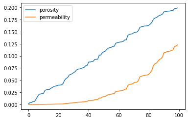
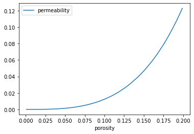
Of course, this is not that useful a plot. What we are likely looking for is a relationship between the DataFrame columns. One way to visualize this is to set the desired abscissa as the DataFrame index and create a plot.

df_new.set_index(['porosity']).plot();

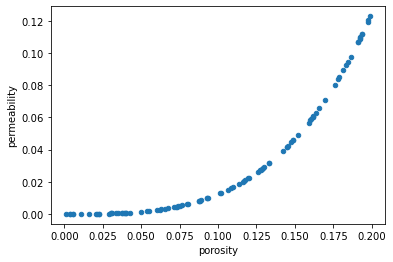
Or explicitly pass the desired independent variable to the x keyword arguments and the dependent variable to the y keyword argument. This time we'll also explicitly create a scatter plot.

When the DataFrame columns are explicitly passed as arguments, the axis labels are correctly populated.

df_new.plot.scatter(x='porosity', y='permeability');

Writing a DataFrame to a File

The most common way way to store and share DataFrames among different computers is the export the DataFrame to a CSV file. This is accomplished with the to_csv member function.

df.to_csv("datasets/200wells_out.csv", index = False)

Displaying the raw data is the file with the UNIX head command

!head -n 5 datasets/200wells_out.csv
Unnamed: 0,X,Y,facies,porosity,perm,ai,% porosity,perm-por ratio,porosity type,perm cutoff,kozeny carmen
38,3505,1525,2,0.2232,174.65400000000002,3.344,22.32,782.5000000000001,high,174.65400000000002,0.18427403135841575
164,2455,2885,2,0.2158,9.592,2.773,21.58,44.44856348470807,high,9.592,0.16341828373836473
148,1975,2745,2,0.2158,361.704,3.839,21.58,1676.1075069508806,high,361.704,0.16341828373836473
97,1855,3025,2,0.2154,463.641,3.091,21.54,2152.465181058496,high,463.641,0.1623455875592409

Further Reading

Further reading on Pandas is avialable in the official Pandas documentation